Introduction
I will begin this article with a pertinent story from my tenure as a mediocre graduate student in Physics. A fellow student and I were working together on a homework set. We had spent the majority of the day on a particularly difficult problem that resulted in a lengthy equation expressed in terms of assorted variables. I turned to the back of the book to compare our result to that of the author's and was astonished by the dissimilarity. I showed the 'correct' solution to my friend, a far better and more confident student than I. After looking at it he asked, "Did we apply the appropriate theorems?" I affirmed that we had. Next, he asked, "Did we make any mathematical errors?" I was confident that we had not. "Then," he proclaimed, "our solution is correct-- we just are expressing it in different terms."
I recall this incident when I encounter a debate over the 'correctness' of the results obtained for particle size measurements by two or more different analytical techniques. Provided that the instruments used are capable of producing high-quality data, the pertinent questions, then, are, “was the sample properly prepared and properly presented to the instrument,” and “were the analytical parameters applied correctly.” If the answer to both is “yes,” then both analytical results probably are equally correct; they are just expressed in different terms.
If what has been stated thus far has not raised any questions, you probably don’t need to read the rest of this article. This article is intended to resolve questions users often have concerning comparisons of particle sizing results by different techniques. The techniques referenced are sieving, sedimentation, imaging (including microscopy and machine vision), electrozone sensing, and light scattering. The determination of particle size on the same sample by all of these techniques and others not mentioned will, in the majority of cases, yield different results for mean size, modal size, and quantity distribution by size.
From the Basics
The following questions may seem simple, but take a close look at the answers. They often contain conditions and constraints that, if not abided by, will affect the accuracy of reported size data.
What defines or characterizes a “particle” and what limitations does the definition impose on particle sizing?
McGraw Hill’s Dictionary of Scientific and Technical Terms (third edition) (1) defines a particle as “any relatively small subdivision of matter, ranging in diameter from a few angstroms to a few millimeters.” Particles that one wishes to measure for size may be composed of organic or inorganic molecules; they may be molecularly homogeneous or inhomogeneous; they may be in solid or liquid state; they may be isotropic or anisotropic; they may be of any shape; and may be suspended in various media. Molecular structure, homogeneity, state, isotropy, shape, and suspension medium associated with the particles under test all may cause different size measurement devices to respond differently to the same particle. When comparing the results from two different types of sizing instruments, one should know if any characteristic of the particle other than size, or any characteristic of the sample presentation could affect the reported size value. Error from these sources is associated with non-ideal or even inappropriate application of the measuring instrument.
Is there a single, standard definition for “particle size” that can be applied to any particle?
There are many definitions, but none has been adopted as a comprehensive standard. To be able to apply a single rule to particle size determinations, and that rule enabling all techniques of sizing to agree is implausible for several reasons. If such a definition is based on geometry it must apply to both regular and irregular shapes and to the techniques used to obtain the measurement. The simplest case in respect to geometry is that of a sphere, and visual inspection (microscopy or image analysis) is the most straightforward measurement technique. When examining a sphere, its perimeter, projected cross-sectional area, surface area, and volume can be described unambiguously by one linear dimension-- the diameter of the projected cross-section. Furthermore, the projected cross-sectional diameter remains constant regardless of the angle of view; therefore a sphere is isotropic in a geometrical sense. No other regular or irregular shape projects the same cross-section at all angles of view, therefore neither surface area nor volume can be inferred from the cross-section of a non spherical particle.
The fact that an irregular particle can present a different cross-section depending on orientation is only one of the measurement problems. Another is that an irregularly shaped cross-section has different “diameters” depending on where the chord is drawn. To deal with these difficulties, definitions of ‘statistical geometric diameters’ were established. They are statistical because they have significance only when averaged over a large number of measurements. An example is Martin’s diameter, which is the length of the chord that divides the cross-sectional shape into two equal areas. Another is Feret’s diameter, which is the distance between two parallel lines tangent to the projected cross-section.
Another approach was to extract a linear size dimension from the projected area of the particle; this is called the ‘area diameter’ and expresses particle size as the diameter of a circle that has the same projected area as the particle. Another was to determine the perimeter of the projected cross-section and assign to the particle the diameter of a circle having the same perimeter. If the volume of an irregular particle could be determined, the diameter of the particle was defined as the diameter of a sphere having the same volume—the volume diameter.
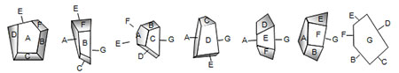
Figure 1. This example particle has seven plane facets, A through G. The particle is shown in seven views, one with each facet parallel to the page. These views represent only a few of the possible orientations and projected cross-sections of the particle. In each, Feret’s diameter, Martin’s diameter, area diameter, and perimeter diameter differ. Only the volume diameter is constant.
Obviously, several different ‘sizes’ could be obtained from a single, non-spherical particle due to various orientations or methods of measurement. Figure 1 is a series of illustrations of the particle; each illustration shows the particle rotated with a different face parallel to the page. Obviously, these are only a few of the possible orientations of the particle, and each orientation projects a different cross-section.
As stated previously, the definitions of particle size are statistical geometric diameters and are applied to large numbers of particles where it is assumed that particles present themselves in random orientations to the measurement system. However, this was found not to be case. A good review of the shortcomings of using these definitions in actual practice is found in Chapter 3 of Mercer’s “Aerosol Technology in Hazard Evaluation”(2).
Without belaboring the subject, it should suffice for the present to state simply that the definition of ‘particle size’ depends on the technique of measurement. Information supporting this is given subsequently.
So, what do particle-sizing instruments actually measure?
Essentially all automated determinations of particle size are obtained indirectly from direct measurements of some parameter other than the complete geometry. These parameters are associated with a physical phenomenon in which the particle is involved. The direct measurement may be of some characteristic of the reaction of the particle to some action, or the measurement may be of the reaction of something that has interacted with the particle. An example of the former is the particle’s sedimentation velocity in a fluid, and of the latter is the pattern of light scattered by the particle. The parameter being directly measured is related to particle geometry by some law, theory or model describing the physical phenomenon.
Table 1 lists classes of particle characteristics related to ‘size’ and to a particular, measurable behavior that varies as a function of particle size. The table also lists other variables that affect the reported size.
| Table 1. Characteristics Associated With Particles and Related to Size |
| Characteristic Class | Behavior or Attribute Related to ‘Size’ | Properties Other Than ‘Size’ That Can Affect the Related Behavior or Attribute | Measurement Techniques Utilizing the Behavior of Attribute |
| Geometrical | Area or perimeter of cross-section | Shape combined with orientation | Microscopy, image recognition, sieving |
| Displacement volume | Porosity, wettability | Electrozone sensing |
| Some linear dimension such as the diameter or statistical geometric diameter | Shape, orientation | Microscopy, image recognition |
| Hydrodynamic / Aerodynamic | Settling velocity Drag (resistance to motion) | Shape and density combined with properties of the surrounding fluid; Reynolds number; molecular homogeneity | Elutriation and sedimentation |
| Optical | Light scattering characteristics | Refractive index, isotropy, shape + orientation, and surface detail of particle. Refractive index of medium. Wavelength and polarity of incident light. | Static light scattering (Mie and Fraunhofer diffraction) |
A comprehensive list of particle sizing techniques is found at Thermo Fisher Scientific's Particle Technology
website.
What is meant by the 'size' of a particle if something other than a geometrical attribute is being measured?
The behavior of a particle or the characteristics of some other entity after interacting with a particle are related to the particle’s geometry, but often in a very complex manner. A common way to describe the geometry of an irregular or regular particle is to compare the particle under test to a sphere of the same material and being of a size that causes it to exhibit the same behavior as the test particle. As an example, when sieving to determine size, the largest particles to pass through the screen are described in terms of the diameter of spheres that will just pass through the same apertures. This is the concept of ‘equivalent spherical size’ and is employed in almost all particle-sizing techniques. An equivalent size may be related to any regular geometry, but the sphere is most often used due to its unique geometrical attributes as previously cited. Another reason for using the sphere as the reference shape in some cases is because the theory describing the behavior of a particle under certain conditions, or describing the results of an interaction with a particle has only been solved rigorously for spherical particles.
Consequently, when reference is made to particles of X mm equivalent spherical diameter, it means that the particles behave (pass through the same size aperture, settle at the same velocity, scatter light with the same intensity at the same angles, or displace the same volume of liquid) as do X mm spherical particles that otherwise have the same behavior-controlling properties as does the sample material.
What has been said about particle sizing above was stated more concisely in the late 1940's by Heywood (3), followed later by Beddow (4). Heywood characterized the results of particle sizing as being ‘somewhat dependent on the physical principles employed and the assumptions or conventions involved.’ He summarized current techniques as being ‘only able to measure and classify particles if the particles under test were imagined as spheres having some property equivalent to the test material.’ Essentially, things are still the same today, and we can add laser diffraction to the list of ‘physical principles employed.’ In the case of laser diffraction, the particles under test are imagined as spheres that scatter light in the same manner as do the particles of the test material.
Since particle sizing techniques apply the common definition of a 'spherical equivalency,' can I expect to get the same measurement results for the same sample from each technique that applies this definition?
If the particles under test are of irregular shape, then the most probable outcome is that the results will differ. Why? Because two particles that, for example, settle with the same velocity (therefore, are the same Stokes size) can scatter light differently (therefore, have different Mie sizes). Two particles that pass through the same screen mesh have the same sieve size, but may have very different volumetric size as determined by electrozone sensing.
If all particles in the sample under test are spherical, then all particle size measuring techniques, in theory, should yield essentially the same results, provided the instrument is applied appropriately. But, being spherical in most cases is only one requirement of the theoretical model. Table 2 lists other assumptions about the particle system that also must be correct. If all of these requirements are satisfied and the value of all other parameters required by the model are known or controlled, then one can expect the results of measurements of a system of spherical particles by different measurement techniques to agree provided that the fundamental measurement data are of comparable quality (precision, accuracy, sensitivity, resolution, signal-to-noise ratio, etc.).
| Table 2. Size Measurement Techniques and the Assumptions of the Theoretical Model |
| Measurement Technique | Model | Assumptions About the Particle System | Other Parameters of the Model |
| Image recognition | Plane geometry | Particles are spherical, cubical or of other regular solid geometry | Known relationship between particle size and image size |
| Electrozone sensing | Ohm's law expressed in terms of electrolyte resistivity, cross-sectional area of aperture, and volume of displaced electrolyte (particle volume) | Spherical particles that are much less conductive than the electrolyte | Size of aperture through which particles pass |
| Sedimentation | Stoke’s Law for the settling velocity of a spherical particle in a fluid medium | Spherical particle, laminar flow of fluid around settling particle, all particles in system of same density | Particle density, density and viscosity of medium at analysis temperature, gravity |
| Static light scattering | Mie theory of light scattering by a spherical particle (includes Fraunhofer theory) | Spherical particle, optically isotropic, no multiple scattering, monochromatic light, coherent light, plane wave | Refractive index of particle, refractive index of medium, wavelength of light, size and position of scattering pattern projected onto detector |
In Table 2, all theoretical models assume spherical particles. What are the effects if the sample particles are not spherical?
Measuring some attribute arising from a non-spherical particle, then reducing the data from those measurements using a spherical model will introduce error—that’s understandable. The magnitude of error depends on the technique and the data reduction method and, of course, the actual shape of the particle compared to the model. As has been mentioned, the mathematical complexities introduced by non-spherical geometry usually prevents models from being derived for other shapes, and these same complexities prevent predicting in exactly what manner the error will affect the reported values. So, depending on the sizing technique and the shape of the particles, the effect may be negligible or may be severe, and often cannot be predicted reliably.
What are the effects on final results if the particles are spherical, but there is some other deviation from the assumptions or conditions of the theoretical model?
Assume that the sedimentation technique is to be used to determine particle size. In this case, the particles’ sedimentation velocities are measured and Stokes’ law is applied. In the application of Stokes’ law, it is assumed that the particle density, liquid density, and liquid viscosity are accurately known. If the value of any of these parameters contains error, say +/- 5%, then the error will affect the calculation of particle size in a predictable manner easily calculable by Stokes law.
A more complex result of deviating from the assumptions of the model occurs in scattered light measurements reduced by Mie theory. A condition of using this theory is that the refractive index of the sample material be known. If the refractive index has an uncertainty of +/-5%, the relationship of this error to the error exhibited in the reported size distribution is considerably more complex. It is unlikely that effects of this error can accurately be predicted, and may only be realized by reducing the experimental data multiple times using a number of values of refractive index covering the range of the uncertainty.
To varying extents, instrument design assures that conditions of the model are met. For example, the requirements for monochromatic and coherent light of a known wavelength for the Mie model in static light scattering instruments is satisfied by the design of the instrument. Determining the density of the sample material, or properly dispersing the sample are examples of experimental conditions that are under the control of the user. In other cases, there are pre-analysis tests to determine if conditions are within the acceptable range of the model. Examples of this are calculating the Reynolds number of the settling particle to assure that it is in the laminar flow domain, or to monitor light extinction as sample concentration is varied to assure that there is neglibible multiple scattering when using the light scattering technique.
In summary, the magnitude of error introduced by deviations from the assumptions of the model or by erroneous parameters depends on the magnitude of the error or degree of deviation, and the ‘sensitivity’ of the data reduction model to these variations. The effect on the reported data ranges from negligible to catastrophic.
Choosing the Right Particle Sizing Instrument for the Application
There is no single sizing technique that is superior in all applications. The instrument selected for an application must be suitable for the material to be measured and for the environment in which the instrument is to be used. It also must provide data to meet the specific needs of the application. This may mean fast, repeatable analyses, or it may mean high-resolution and very accurate results. The determination of particle size distribution seldom is the ultimate objective; determining how particle size affects something else is usually the reason for the measurement. In this regard, the characteristic actually being measured and related to size may be more important than size, but size is the best way or the conventional way to express the characteristic. For example, sediment from an extinct river delta may be analyzed for size. But, what actually may be of interest is the deposition mechanism. In this case, size is a way of expressing sedimentation velocity and the sedimentation size (Stokes size) may be of more value than the size determined by light scattering (Mie size).
Literally, the bottom line is this: Different techniques are likely to produce different size results for the same particle, and all of them are likely to be correct. The best instrument for the application (the best size definition) may be the one that most closely relates particle size to the application of the particles.
References:
- Dictionary of Scientific and Technical Terms, Third Ed., McGraw Hill Book Company, N.Y. (1984).
- Mercer, Thomas T., Aerosol Technology in Hazard Evaluation, Academic Press, N.Y. (1973).
- Harold Heywood, The Scope of Particle Size Analysis and Standardization, Institution of Chemical Engineers, Symposium on Particle Size Analysis (1947).
- Beddow, John Keith, On the Design of a System for Particle Shape Analysis, College of Engineering, Materials Engineering Division, The University of Iowa, Report NSF-76-004 (1976).
Web sites containing information of particle sizing:
Recommended reading:
Sizing techniques, surface area, and porosimetry: Allen, Terence, Particle Size Measurement, Chapman and Hall (1990)
Geological applications: Syvitski, James P.M., Principles, Methods, and Application of Particle Size Analysis, Cambridge University Press (1991)
Sizing techniques: Provder, Theodore, Particle Size Distribution II Assessment and Characterization, Oxford University Press
Standard Test Methods:
ASTM
B330-88(1993)e1 Standard Test Method for Average Particle Size of Powders of Refractory Metals and Their Compounds by the Fisher
Sub-Sieve Sizer
B430-97 Standard Test Method for Particle Size Distribution of Refractory Metal Powders and Related Compounds by Turbidimetry
B761-97 Standard Test Method for Particle Size Distribution of Refractory Metals and Their Compounds by X-Ray Monitoring of Gravity Sedimentation
B821-92 Standard Guide for Liquid Dispersion of Metal Powders and Related Compounds for Particle Size Analysis
B822-92 Standard Test Method for Particle Size Distribution of Metal Powders and Related Compounds by Light Scattering
B859-95 Standard Practice for De-Agglomeration of Refractory Metal Powders and Their Compounds Prior to Particle Size Analysis
C1070-86e1 Standard Test Method for Determining Particle Size Distribution of Alumina or Quartz by Laser Light Scattering
C1182-91(1995) Standard Test Method for Determining the Particle Size Distribution of Alumina by Centrifugal Photosedimentation
C1282-94 Standard Test Method for Determining the Particle Size Distribution of Advanced Ceramics by Centrifugal Photosedimentation
C690-86(1997)e1 Standard Test Method for Particle Size Distribution of Alumina or Quartz by Electric Sensing Zone Technique
C721-81(1997)e1 Standard Test Method for Average Particle Size of Alumina and Silica Powders by Air Permeability
C958-92(1997)e1 Standard Test Method for Particle Size Distribution of Alumina or Quartz by X-Ray Monitoring of Gravity Sedimentation
D1366-86(1997) Standard Practice for Reporting Particle Size Characteristics of Pigments
D1705-92 Standard Test Method for Particle Size Analysis of Powdered Polymers and Copolymers of Vinyl Chloride
D1921-96 Standard Test Methods for Particle Size (Sieve Analysis) of Plastic Materials
D2338-84(1989)e1 Standard Test Method for Determining Particle Size of Multicolor Lacquers
D2862-92 Standard Test Method for Particle Size Distribution of Granular Activated Carbon
D2977-71(1996) Standard Test Method for Particle Size Range of Peat Materials for Horticultural Purposes
D3360-96 Standard Test Method for Particle Size Distribution by Hydrometer of the Common White Extender Pigments
D4438-85 Standard Test Method for Particle Size Distribution of Catalytic Material by Electronic Counting
D4464-85 Standard Test Method for Particle Size Distribution of Catalytic Material by Laser Light Scattering
D4513-97 Standard Test Method for Particle Size Distribution of Catalytic Materials by Sieving
D4570-86(1993)e1 Standard Test Method for Rubber Chemicals-Determination of Particle Size of Sulfur by Sieving (Dry)
D4822-88(1994)e1 Standard Guide for Selection of Methods of Particle Size Analysis of Fluvial Sediments (Manual Methods)
D502-89(1995)e1 Standard Test Method for Particle Size of Soaps and Other Detergents
D5158-93 Standard Test Method for Determination of the Particle Size of Powdered Activated Carbon
D5519-94 Standard Test Method for Particle Size Analysis of Natural and Man-Made Riprap Materials
D5644-96 Standard Test Method for Rubber Compounding Materials-Determination of Particle Size Distribution of Vulcanized Particulate Rubber
D5861-95 Standard Guide for Significance of Particle Size Measurements of Coating Powders
E1037-84(1996)e1 Standard Test Method for Measuring Particle Size Distribution of RDF-5
E1617-97 Standard Practice for Reporting Particle Size Characterization Data
E1772-95 Standard Test Method for Particle Size Distribution of Chromatography Media by Electric Sensing Zone Technique
E276-93 Standard Test Method for Particle Size or Screen Analysis at No. 4 (4.75-mm) Sieve and Finer for Metal-Bearing Ores and
Related Materials
E389-93(1998) Standard Test Method for Particle Size or Screen Analysis at No. 4 (4.75-mm) Sieve and Coarser for Metal-Bearing Ores and
Related Materials
E726-96 Standard Test Method for Particle Size Distribution of Granular Carriers and Granular Pesticides
F1632-95 Standard Test Method for Particle Size Analysis and Sand Shape Grading of Golf Course Putting Green and Sports Field
Rootzone Mixes
F577-83(1993)e1 Standard Test Method for Particle Size Measurement of Dry Toners
F660-83(1993) Standard Practice for Comparing Particle Size in the Use of Alternative Types of Particle Counters
F751-83(1993)e1 Standard Test Method for Measuring Particle Size of Wide-Size Range Dry Toners
ISO
ISO 643:1983 Steels -- Micrographic determination of the ferritic or austenitic grain size
ISO 728:1995 Coke (nominal top size greater than 20 mm) -- Size analysis by sieving
ISO 1953:1994 Hard coal -- Size analysis by sieving
ISO 2030:1990 Granulated cork -- Size analysis by mechanical sieving
ISO 2325:1986 Coke -- Size analysis (Nominal top size 20 mm or less)
ISO 2926:1974 Aluminium oxide primarily used for the production of aluminium -- Particle size analysis --Sieving method
ISO 2996:1974 Sodium tripolyphosphate and sodium pyrophosphate for industrial use -- Determination of particle size distribution by mechanical sieving
?ISO 3118:1976 Sodium perborates for industrial use -- Determination of particle size distribution by mechanical sieving
ISO 4150:1991 Green coffee -- Size analysis -- Manual sieving
ISO 4497:1983 Metallic powders -- Determination of particle size by dry sieving
ISO 4701:1999 Iron ores -- Determination of size distribution by sieving
ISO 4783-1:1989 Industrial wire screens and woven wire cloth -- Guide to the choice of aperture size and wire diameter combinations -- Part 1: Generalities
ISO 5915:1980 Sodium hexafluorosilicate for industrial use -- Determination of particle size distribution -- Sieving method
ISO 6230:1989 Manganese ores -- Determination of size distribution by sieving
ISO 6344-1:1998 Coated abrasives -- Grain size analysis -- Part 1: Grain size distribution test
ISO 6344-2:1998 Coated abrasives -- Grain size analysis -- Part 2: Determination of grain size distribution of macrogrits P12 to P220
ISO 6344-3:1998 Coated abrasives -- Grain size analysis -- Part 3: Determination of grain size distribution of microgrits P240 to P2500
ISO 7532:1985 Instant coffee -- Size analysis
ISO 8130-1:1992 Coating powders -- Part 1: Determination of particle size distribution by sieving
ISO 8220:1986 Aluminium oxide primarily used for the production of aluminium -- Determination of the fine particle size distribution (less than 60 mu/m) -- Method using electroformed sieves
ISO 8486-1:1996 Bonded abrasives -- Determination and designation of grain size distribution -- Part 1: Macrogrits F4 to F220
ISO 8486-2:1996 Bonded abrasives -- Determination and designation of grain size distribution -- Part 2: Microgrits F230 to F1200
ISO 8511:1995 Rubber compounding ingredients -- Carbon black -- Determination of pellet size distribution
ISO 8876:1989 Fluorspar -- Determination of particle size distribution by sieving
ISO 9276-1:1998 Representation of results of particle size analysis -- Part 1: Graphical representation
ISO 10076:1991 Metallic powders -- Determination of particle size distribution by gravitational sedimentation in a liquid and attenuation measurement
ISO 11125-2:1993 Preparation of steel substrates before application of paints and related products – Test methods for metallic blast-cleaning abrasives -- Part 2: Determination of particle size distribution
ISO 11127-2:1993 Preparation of steel substrates before application of paints and related products – Test methods for non-metallic blast-cleaning abrasives -- Part 2: Determination of particle size distribution
ISO 11277:1998 Soil quality -- Determination of particle size distribution in mineral soil material – Method by sieving and sedimentation
ISO 12984:2000 Carbonaceous materials used in the production of aluminium -- Calcined coke -- Determination of particle size distribution
ISO 13319:2000 Determination of particle size distributions -- Electrical sensing zone method
ISO 13320-1:1999 Particle size analysis -- Laser diffraction methods -- Part 1: General principles
ISO 13321:1996 Particle size analysis -- Photon correlation spectroscopy
ISO 13366-2:1997 Milk -- Enumeration of somatic cells -- Part 2: Electronic particle counter method
ISO 14703:2000 Fine ceramics (advanced ceramics, advanced technical ceramics) -- Sample preparation for the determination of particle size distribution of ceramic powders